Sharath Kannan and Greg Dellamura
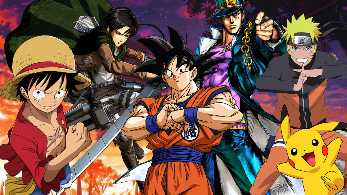
Anime is hand-drawn and computer-generated animation that originated in Japan. In English terms, Anime is referred to as Japanese animation, but in Japanese terms, Anime is referred to as general animation. The origin of anime can be traced back all the way to 1917 but it didn’t really obtain an identity until the 1960s when anime began to start gaining a bigger audience and has become increasingly popular over the past decade or two. Most of the time, Anime can be an adaptation of manga (Japanese comics), light novels, and video games. Some popular examples of anime are Pokemon, Naruto, Dragon Ball, Attack on Titan, and Demon Slayer.
Compared to Western Animation, the Art style is very diverse with characters where their features can vary. The most iconic characteristic of anime characters is their large and emotive eyes. The animation also focuses less on movement and more on the detail of settings and camera effects.
The main question we will be answering is if the popularity of anime is determined by factors not on the quality of the anime, such as the season it was released in, the number of episodes it has, or if it falls into a certain genre group.
Data was obtained from Kaggle.com which web scraped MyAnimeList.net. MyAnimeList is a website run by volunteers that social network and catalog based on anime and manga. The site provides a list of all anime and manga that members can personally organize and score. In 2015, the site received 120 million visitors a month. This dataset has been compiled on Kaggle: https://www.kaggle.com/datasets/harits/anime-database-2022
#from google.colab import drive
#drive.mount('/content/drive')
import pandas as pd
import matplotlib.pyplot as plt
import seaborn as sb
import numpy as np
from datetime import datetime as dt
import re
# supress uneccessary warning
pd.options.mode.chained_assignment = None # default='warn'
an_df = pd.read_csv("AnimeRecent.csv")
The dataset has many unwanted features and values not in the right format to answer our hypothesis. We need to make sure the dataset is ready for data analysis and model use.
an_df = an_df.drop(["Synopsis", "Synonyms", "Japanese", "ID", "Status"], axis=1)
an_df.head()
Title | English | Type | Episodes | Start_Aired | End_Aired | Premiered | Broadcast | Producers | Licensors | ... | Themes | Demographics | Duration_Minutes | Rating | Score | Scored_Users | Ranked | Popularity | Members | Favorites | |
---|---|---|---|---|---|---|---|---|---|---|---|---|---|---|---|---|---|---|---|---|---|
0 | Shingeki no Kyojin | Attack on Titan | TV | 25.0 | Apr 7, 2013 | Sep 29, 2013 | Spring 2013 | Sundays at 0158 (JST) | Production I.G, Dentsu, Mainichi Broadcasting ... | Funimation | ... | Gore, Military, Survival | Shounen | 24.0 | R - 17+ (violence & profanity) | 8.531 | 519803.0 | 1002.0 | 1 | 3524109 | 155695 |
1 | Death Note | Death Note | TV | 37.0 | Oct 4, 2006 | Jun 27, 2007 | Fall 2006 | Wednesdays at 0056 (JST) | VAP, Konami, Ashi Productions, Nippon Televisi... | VIZ Media | ... | Psychological | Shounen | 23.0 | R - 17+ (violence & profanity) | 8.621 | 485487.0 | 732.0 | 2 | 3504535 | 159701 |
2 | Fullmetal Alchemist: Brotherhood | Fullmetal Alchemist Brotherhood | TV | 64.0 | Apr 5, 2009 | Jul 4, 2010 | Spring 2009 | Sundays at 1700 (JST) | Aniplex, Square Enix, Mainichi Broadcasting Sy... | Funimation, Aniplex of America | ... | Military | Shounen | 24.0 | R - 17+ (violence & profanity) | 9.131 | 900398.0 | 12.0 | 3 | 2978455 | 207772 |
3 | One Punch Man | One Punch Man | TV | 12.0 | Oct 5, 2015 | Dec 21, 2015 | Fall 2015 | Mondays at 0105 (JST) | TV Tokyo, Bandai Visual, Lantis, Asatsu DK, Ba... | VIZ Media | ... | Parody, Super Power | Seinen | 24.0 | R - 17+ (violence & profanity) | 8.511 | 19066.0 | 1112.0 | 4 | 2879907 | 59651 |
4 | Sword Art Online | Sword Art Online | TV | 25.0 | Jul 8, 2012 | Dec 23, 2012 | Summer 2012 | Sundays at 0000 (JST) | Aniplex, Genco, DAX Production, ASCII Media Wo... | Aniplex of America | ... | Love Polygon, Video Game | Unknown | 23.0 | PG-13 - Teens 13 or older | 7.201 | 990254.0 | 29562.0 | 5 | 2813565 | 64997 |
5 rows × 23 columns
We want to drop Synopsis, Synonyms, Japanese, ID, and Status because they serve no purpose to our hypothesis
#Remove Music Type
an_df.loc[an_df['Type'] == 'Music'] = np.NaN
#Remove Unknown Type
an_df.loc[an_df['Type'] == 'Unknown'] = np.NaN
an_df = an_df.dropna()
an_df.head()
Title | English | Type | Episodes | Start_Aired | End_Aired | Premiered | Broadcast | Producers | Licensors | ... | Themes | Demographics | Duration_Minutes | Rating | Score | Scored_Users | Ranked | Popularity | Members | Favorites | |
---|---|---|---|---|---|---|---|---|---|---|---|---|---|---|---|---|---|---|---|---|---|
0 | Shingeki no Kyojin | Attack on Titan | TV | 25.0 | Apr 7, 2013 | Sep 29, 2013 | Spring 2013 | Sundays at 0158 (JST) | Production I.G, Dentsu, Mainichi Broadcasting ... | Funimation | ... | Gore, Military, Survival | Shounen | 24.0 | R - 17+ (violence & profanity) | 8.531 | 519803.0 | 1002.0 | 1.0 | 3524109.0 | 155695.0 |
1 | Death Note | Death Note | TV | 37.0 | Oct 4, 2006 | Jun 27, 2007 | Fall 2006 | Wednesdays at 0056 (JST) | VAP, Konami, Ashi Productions, Nippon Televisi... | VIZ Media | ... | Psychological | Shounen | 23.0 | R - 17+ (violence & profanity) | 8.621 | 485487.0 | 732.0 | 2.0 | 3504535.0 | 159701.0 |
2 | Fullmetal Alchemist: Brotherhood | Fullmetal Alchemist Brotherhood | TV | 64.0 | Apr 5, 2009 | Jul 4, 2010 | Spring 2009 | Sundays at 1700 (JST) | Aniplex, Square Enix, Mainichi Broadcasting Sy... | Funimation, Aniplex of America | ... | Military | Shounen | 24.0 | R - 17+ (violence & profanity) | 9.131 | 900398.0 | 12.0 | 3.0 | 2978455.0 | 207772.0 |
3 | One Punch Man | One Punch Man | TV | 12.0 | Oct 5, 2015 | Dec 21, 2015 | Fall 2015 | Mondays at 0105 (JST) | TV Tokyo, Bandai Visual, Lantis, Asatsu DK, Ba... | VIZ Media | ... | Parody, Super Power | Seinen | 24.0 | R - 17+ (violence & profanity) | 8.511 | 19066.0 | 1112.0 | 4.0 | 2879907.0 | 59651.0 |
4 | Sword Art Online | Sword Art Online | TV | 25.0 | Jul 8, 2012 | Dec 23, 2012 | Summer 2012 | Sundays at 0000 (JST) | Aniplex, Genco, DAX Production, ASCII Media Wo... | Aniplex of America | ... | Love Polygon, Video Game | Unknown | 23.0 | PG-13 - Teens 13 or older | 7.201 | 990254.0 | 29562.0 | 5.0 | 2813565.0 | 64997.0 |
5 rows × 23 columns
We want to get change "Unkown" Anime Type to NaN because it is easier to work with when plotting. We also changed Music to NaN because we do not want Anime Music to be apart of our analysis
an_df = an_df.replace('R - 17+ (violence & profanity)', 'R-17+')
an_df = an_df.replace('PG-13 - Teens 13 or older', 'PG-13')
an_df = an_df.replace('R+ - Mild Nudity', 'R+')
an_df = an_df.replace('G - All Ages', 'G')
an_df = an_df.replace('PG - Children', 'PG')
an_df = an_df.replace('None', 'NR')
an_df.head()
Title | English | Type | Episodes | Start_Aired | End_Aired | Premiered | Broadcast | Producers | Licensors | ... | Themes | Demographics | Duration_Minutes | Rating | Score | Scored_Users | Ranked | Popularity | Members | Favorites | |
---|---|---|---|---|---|---|---|---|---|---|---|---|---|---|---|---|---|---|---|---|---|
0 | Shingeki no Kyojin | Attack on Titan | TV | 25.0 | Apr 7, 2013 | Sep 29, 2013 | Spring 2013 | Sundays at 0158 (JST) | Production I.G, Dentsu, Mainichi Broadcasting ... | Funimation | ... | Gore, Military, Survival | Shounen | 24.0 | R-17+ | 8.531 | 519803.0 | 1002.0 | 1.0 | 3524109.0 | 155695.0 |
1 | Death Note | Death Note | TV | 37.0 | Oct 4, 2006 | Jun 27, 2007 | Fall 2006 | Wednesdays at 0056 (JST) | VAP, Konami, Ashi Productions, Nippon Televisi... | VIZ Media | ... | Psychological | Shounen | 23.0 | R-17+ | 8.621 | 485487.0 | 732.0 | 2.0 | 3504535.0 | 159701.0 |
2 | Fullmetal Alchemist: Brotherhood | Fullmetal Alchemist Brotherhood | TV | 64.0 | Apr 5, 2009 | Jul 4, 2010 | Spring 2009 | Sundays at 1700 (JST) | Aniplex, Square Enix, Mainichi Broadcasting Sy... | Funimation, Aniplex of America | ... | Military | Shounen | 24.0 | R-17+ | 9.131 | 900398.0 | 12.0 | 3.0 | 2978455.0 | 207772.0 |
3 | One Punch Man | One Punch Man | TV | 12.0 | Oct 5, 2015 | Dec 21, 2015 | Fall 2015 | Mondays at 0105 (JST) | TV Tokyo, Bandai Visual, Lantis, Asatsu DK, Ba... | VIZ Media | ... | Parody, Super Power | Seinen | 24.0 | R-17+ | 8.511 | 19066.0 | 1112.0 | 4.0 | 2879907.0 | 59651.0 |
4 | Sword Art Online | Sword Art Online | TV | 25.0 | Jul 8, 2012 | Dec 23, 2012 | Summer 2012 | Sundays at 0000 (JST) | Aniplex, Genco, DAX Production, ASCII Media Wo... | Aniplex of America | ... | Love Polygon, Video Game | Unknown | 23.0 | PG-13 | 7.201 | 990254.0 | 29562.0 | 5.0 | 2813565.0 | 64997.0 |
5 rows × 23 columns
We want to simplify and reduce the ratings of the Anime by removing the reasoning for the ratings to make the plots easier to read and look nicer
an_df = an_df.replace('Kids, Shounen', 'Shounen')
an_df = an_df.replace('Kids, Shoujo', 'Shoujo')
an_df = an_df.replace('Josei, Shoujo', 'Shoujo')
an_df = an_df.replace('Kids, Seinen', 'Seinen')
an_df.head()
Title | English | Type | Episodes | Start_Aired | End_Aired | Premiered | Broadcast | Producers | Licensors | ... | Themes | Demographics | Duration_Minutes | Rating | Score | Scored_Users | Ranked | Popularity | Members | Favorites | |
---|---|---|---|---|---|---|---|---|---|---|---|---|---|---|---|---|---|---|---|---|---|
0 | Shingeki no Kyojin | Attack on Titan | TV | 25.0 | Apr 7, 2013 | Sep 29, 2013 | Spring 2013 | Sundays at 0158 (JST) | Production I.G, Dentsu, Mainichi Broadcasting ... | Funimation | ... | Gore, Military, Survival | Shounen | 24.0 | R-17+ | 8.531 | 519803.0 | 1002.0 | 1.0 | 3524109.0 | 155695.0 |
1 | Death Note | Death Note | TV | 37.0 | Oct 4, 2006 | Jun 27, 2007 | Fall 2006 | Wednesdays at 0056 (JST) | VAP, Konami, Ashi Productions, Nippon Televisi... | VIZ Media | ... | Psychological | Shounen | 23.0 | R-17+ | 8.621 | 485487.0 | 732.0 | 2.0 | 3504535.0 | 159701.0 |
2 | Fullmetal Alchemist: Brotherhood | Fullmetal Alchemist Brotherhood | TV | 64.0 | Apr 5, 2009 | Jul 4, 2010 | Spring 2009 | Sundays at 1700 (JST) | Aniplex, Square Enix, Mainichi Broadcasting Sy... | Funimation, Aniplex of America | ... | Military | Shounen | 24.0 | R-17+ | 9.131 | 900398.0 | 12.0 | 3.0 | 2978455.0 | 207772.0 |
3 | One Punch Man | One Punch Man | TV | 12.0 | Oct 5, 2015 | Dec 21, 2015 | Fall 2015 | Mondays at 0105 (JST) | TV Tokyo, Bandai Visual, Lantis, Asatsu DK, Ba... | VIZ Media | ... | Parody, Super Power | Seinen | 24.0 | R-17+ | 8.511 | 19066.0 | 1112.0 | 4.0 | 2879907.0 | 59651.0 |
4 | Sword Art Online | Sword Art Online | TV | 25.0 | Jul 8, 2012 | Dec 23, 2012 | Summer 2012 | Sundays at 0000 (JST) | Aniplex, Genco, DAX Production, ASCII Media Wo... | Aniplex of America | ... | Love Polygon, Video Game | Unknown | 23.0 | PG-13 | 7.201 | 990254.0 | 29562.0 | 5.0 | 2813565.0 | 64997.0 |
5 rows × 23 columns
when an anime has more than one Demographic, we reduced it to the more major type. Shounen and Shoujo are the two most popular
#Extracting the Season and Year of the Premiere and make their own seperate columns
an_df = an_df.assign(Season=np.nan)
an_df = an_df.assign(Year=np.nan)
for i in range(0, len(an_df['Premiered'])):
premiered = an_df['Premiered'].iloc[i]
if 'Spring' in premiered :
an_df['Season'].iloc[i] = 'Spring'
elif 'Fall' in premiered :
an_df['Season'].iloc[i] = 'Fall'
elif 'Winter' in premiered :
an_df['Season'].iloc[i] = 'Winter'
elif 'Summer' in premiered :
an_df['Season'].iloc[i] = 'Summer'
if 'Unknown' in premiered :
an_df['Season'].iloc[i] = 'Unknown'
an_df['Year'].iloc[i] = 'Unknown'
else :
an_df['Year'].iloc[i] = premiered[len(premiered) - 4 : len(premiered)]
an_df = an_df.drop(["Premiered"], axis = 1)
an_df.head()
Title | English | Type | Episodes | Start_Aired | End_Aired | Broadcast | Producers | Licensors | Studios | ... | Duration_Minutes | Rating | Score | Scored_Users | Ranked | Popularity | Members | Favorites | Season | Year | |
---|---|---|---|---|---|---|---|---|---|---|---|---|---|---|---|---|---|---|---|---|---|
0 | Shingeki no Kyojin | Attack on Titan | TV | 25.0 | Apr 7, 2013 | Sep 29, 2013 | Sundays at 0158 (JST) | Production I.G, Dentsu, Mainichi Broadcasting ... | Funimation | Wit Studio | ... | 24.0 | R-17+ | 8.531 | 519803.0 | 1002.0 | 1.0 | 3524109.0 | 155695.0 | Spring | 2013 |
1 | Death Note | Death Note | TV | 37.0 | Oct 4, 2006 | Jun 27, 2007 | Wednesdays at 0056 (JST) | VAP, Konami, Ashi Productions, Nippon Televisi... | VIZ Media | Madhouse | ... | 23.0 | R-17+ | 8.621 | 485487.0 | 732.0 | 2.0 | 3504535.0 | 159701.0 | Fall | 2006 |
2 | Fullmetal Alchemist: Brotherhood | Fullmetal Alchemist Brotherhood | TV | 64.0 | Apr 5, 2009 | Jul 4, 2010 | Sundays at 1700 (JST) | Aniplex, Square Enix, Mainichi Broadcasting Sy... | Funimation, Aniplex of America | Bones | ... | 24.0 | R-17+ | 9.131 | 900398.0 | 12.0 | 3.0 | 2978455.0 | 207772.0 | Spring | 2009 |
3 | One Punch Man | One Punch Man | TV | 12.0 | Oct 5, 2015 | Dec 21, 2015 | Mondays at 0105 (JST) | TV Tokyo, Bandai Visual, Lantis, Asatsu DK, Ba... | VIZ Media | Madhouse | ... | 24.0 | R-17+ | 8.511 | 19066.0 | 1112.0 | 4.0 | 2879907.0 | 59651.0 | Fall | 2015 |
4 | Sword Art Online | Sword Art Online | TV | 25.0 | Jul 8, 2012 | Dec 23, 2012 | Sundays at 0000 (JST) | Aniplex, Genco, DAX Production, ASCII Media Wo... | Aniplex of America | A-1 Pictures | ... | 23.0 | PG-13 | 7.201 | 990254.0 | 29562.0 | 5.0 | 2813565.0 | 64997.0 | Summer | 2012 |
5 rows × 24 columns
Next we decided to split the Premiered column into two separate columns, Season and Year to make it easier to work with the data and use it for plotting. Majority of anime releases based on the seasons of the year, Spring, Summer, Fall, and Winter.
an_df['Demographics'].loc[an_df['Demographics'] == 'Unknown'] = np.NaN #Convert Unknown Demographics to NaN
an_df.head()
Title | English | Type | Episodes | Start_Aired | End_Aired | Broadcast | Producers | Licensors | Studios | ... | Duration_Minutes | Rating | Score | Scored_Users | Ranked | Popularity | Members | Favorites | Season | Year | |
---|---|---|---|---|---|---|---|---|---|---|---|---|---|---|---|---|---|---|---|---|---|
0 | Shingeki no Kyojin | Attack on Titan | TV | 25.0 | Apr 7, 2013 | Sep 29, 2013 | Sundays at 0158 (JST) | Production I.G, Dentsu, Mainichi Broadcasting ... | Funimation | Wit Studio | ... | 24.0 | R-17+ | 8.531 | 519803.0 | 1002.0 | 1.0 | 3524109.0 | 155695.0 | Spring | 2013 |
1 | Death Note | Death Note | TV | 37.0 | Oct 4, 2006 | Jun 27, 2007 | Wednesdays at 0056 (JST) | VAP, Konami, Ashi Productions, Nippon Televisi... | VIZ Media | Madhouse | ... | 23.0 | R-17+ | 8.621 | 485487.0 | 732.0 | 2.0 | 3504535.0 | 159701.0 | Fall | 2006 |
2 | Fullmetal Alchemist: Brotherhood | Fullmetal Alchemist Brotherhood | TV | 64.0 | Apr 5, 2009 | Jul 4, 2010 | Sundays at 1700 (JST) | Aniplex, Square Enix, Mainichi Broadcasting Sy... | Funimation, Aniplex of America | Bones | ... | 24.0 | R-17+ | 9.131 | 900398.0 | 12.0 | 3.0 | 2978455.0 | 207772.0 | Spring | 2009 |
3 | One Punch Man | One Punch Man | TV | 12.0 | Oct 5, 2015 | Dec 21, 2015 | Mondays at 0105 (JST) | TV Tokyo, Bandai Visual, Lantis, Asatsu DK, Ba... | VIZ Media | Madhouse | ... | 24.0 | R-17+ | 8.511 | 19066.0 | 1112.0 | 4.0 | 2879907.0 | 59651.0 | Fall | 2015 |
4 | Sword Art Online | Sword Art Online | TV | 25.0 | Jul 8, 2012 | Dec 23, 2012 | Sundays at 0000 (JST) | Aniplex, Genco, DAX Production, ASCII Media Wo... | Aniplex of America | A-1 Pictures | ... | 23.0 | PG-13 | 7.201 | 990254.0 | 29562.0 | 5.0 | 2813565.0 | 64997.0 | Summer | 2012 |
5 rows × 24 columns
Next we changed 'Unknown' Demographics to NaN to make it easier to work with
#Reorder Columns
an_df = an_df[['Title', 'English', 'Type', 'Episodes', 'Duration_Minutes', 'Season', 'Year',
'Broadcast', 'Producers', 'Licensors', 'Studios', 'Source', 'Genres', 'Themes', 'Demographics',
'Rating', 'Score', 'Scored_Users', 'Ranked', 'Popularity', 'Members', 'Favorites']]
an_df = an_df.reset_index(drop=True)
an_df.head()
Title | English | Type | Episodes | Duration_Minutes | Season | Year | Broadcast | Producers | Licensors | ... | Genres | Themes | Demographics | Rating | Score | Scored_Users | Ranked | Popularity | Members | Favorites | |
---|---|---|---|---|---|---|---|---|---|---|---|---|---|---|---|---|---|---|---|---|---|
0 | Shingeki no Kyojin | Attack on Titan | TV | 25.0 | 24.0 | Spring | 2013 | Sundays at 0158 (JST) | Production I.G, Dentsu, Mainichi Broadcasting ... | Funimation | ... | Action, Drama | Gore, Military, Survival | Shounen | R-17+ | 8.531 | 519803.0 | 1002.0 | 1.0 | 3524109.0 | 155695.0 |
1 | Death Note | Death Note | TV | 37.0 | 23.0 | Fall | 2006 | Wednesdays at 0056 (JST) | VAP, Konami, Ashi Productions, Nippon Televisi... | VIZ Media | ... | Supernatural, Suspense | Psychological | Shounen | R-17+ | 8.621 | 485487.0 | 732.0 | 2.0 | 3504535.0 | 159701.0 |
2 | Fullmetal Alchemist: Brotherhood | Fullmetal Alchemist Brotherhood | TV | 64.0 | 24.0 | Spring | 2009 | Sundays at 1700 (JST) | Aniplex, Square Enix, Mainichi Broadcasting Sy... | Funimation, Aniplex of America | ... | Action, Adventure, Drama, Fantasy | Military | Shounen | R-17+ | 9.131 | 900398.0 | 12.0 | 3.0 | 2978455.0 | 207772.0 |
3 | One Punch Man | One Punch Man | TV | 12.0 | 24.0 | Fall | 2015 | Mondays at 0105 (JST) | TV Tokyo, Bandai Visual, Lantis, Asatsu DK, Ba... | VIZ Media | ... | Action, Comedy | Parody, Super Power | Seinen | R-17+ | 8.511 | 19066.0 | 1112.0 | 4.0 | 2879907.0 | 59651.0 |
4 | Sword Art Online | Sword Art Online | TV | 25.0 | 23.0 | Summer | 2012 | Sundays at 0000 (JST) | Aniplex, Genco, DAX Production, ASCII Media Wo... | Aniplex of America | ... | Action, Adventure, Fantasy, Romance | Love Polygon, Video Game | NaN | PG-13 | 7.201 | 990254.0 | 29562.0 | 5.0 | 2813565.0 | 64997.0 |
5 rows × 22 columns
Next we reordered the columns and reset the index to clean up the dataframe
The first thing we decided to do is to use df.describe() to gain basic insight on the dataset.
an_df.describe()
Episodes | Duration_Minutes | Score | Scored_Users | Ranked | Popularity | Members | Favorites | |
---|---|---|---|---|---|---|---|---|
count | 11832.000000 | 11832.000000 | 11832.000000 | 11832.000000 | 11832.000000 | 11832.000000 | 1.183200e+04 | 11832.000000 |
mean | 13.749070 | 28.218729 | 6.517990 | 32064.138861 | 63033.302400 | 6995.155088 | 6.902013e+04 | 810.682387 |
std | 54.844314 | 26.511146 | 0.919228 | 93279.255883 | 37539.391852 | 4463.040989 | 2.050284e+05 | 5685.765462 |
min | 1.000000 | 1.000000 | 1.841000 | 102.000000 | 12.000000 | 1.000000 | 1.920000e+02 | 0.000000 |
25% | 1.000000 | 11.000000 | 5.921000 | 491.000000 | 30539.500000 | 3046.750000 | 1.533750e+03 | 1.000000 |
50% | 3.000000 | 24.000000 | 6.531000 | 2578.500000 | 61927.000000 | 6616.000000 | 6.950500e+03 | 10.000000 |
75% | 13.000000 | 28.000000 | 7.181000 | 17433.000000 | 94624.500000 | 10811.500000 | 4.067675e+04 | 92.000000 |
max | 3057.000000 | 168.000000 | 9.131000 | 997243.000000 | 131202.000000 | 17677.000000 | 3.524109e+06 | 207772.000000 |
an_df.describe() gives us a basic breakdown of various summary stats of the numerical columns in the dataset. Here are some important insights that we've garnered from this:
Afterwards, we decided to create a heatmap of all the columns to see which features interact with each other and how strong the correlations are.
fig, ax = plt.subplots(figsize=(8,8))
an_corr = an_df.corr() #Computes correlation of columns, excluding NaN values
an_heatmap = sb.heatmap(an_corr, ax=ax, annot=True, fmt=".2f", linewidths=.5, vmin=0, vmax=1)
None
This Heat Map shows if there is a correlation between Episodes, Score, Scored_Users, Ranking, Popularity, # of Members, and # of Favorited by Members. All green cells in the heat map represent that there is little to no correlation between the two categories. Cells that are blue show that there is somewhat of a correlation between the two categories. From Highest to Lowest Correlation we have:
We decided to ignore the Ranked, Scored_Users, Popularity, Members, and Favorites column because they served no purpose for our hypothesis.
Machine Learning models are not well-suited for categorical data labeled with String objects. Therefore, it is in best interest to One-Hot encode the data. This essentially means creating a new feature and column based on the category. If the row supports the feature, the value in the new column is set to one. If now, the value is set to two. Now, all of our categorical data is easily interpretable by models.
In the Anime Dataset, the Themes, Genres, and Studio columns have categories. The oneHot_encode_col() function below takes any of these columns and creates a new dataframe with one-hot encoded data. This dataframe can then be attatched to the main an_df to be trained with a model.
Each column has a list of categories sepereted by a delimiter: ", ". By splitting the String using the split() function, we are able to get a list of categories for a particular row. First, we get a list of all unique categories in the column. We store this in a dictionary where the keys are the category name, and the column will be a list of size len(an_df). Second, we fill that list with ones and zeroes depending on if the category exists in that specific row or not. Finally, we return the new dataframe.
The one-hot encoded dataframe can also double as a count of certain categories. In the previous dataset, this was not possible.
# oneHot_encode_col(col)
# This can one-hot enode any column with categories
# creating a dataframe with binary values (1 and 0)
# in this dataset, categories are split with ", "
def oneHot_encode_col(col):
# create a list of all categories
all_cats = {}
for cat_info in an_df[col]:
splt = cat_info.split(", ")
for cat in splt:
if (cat in all_cats):
pass
else:
all_cats[cat] = []
# for testing purposes
# print(all_cats)
# if the column has a speific category,
# it lables that row with a 1. else, it
# lables that category with a 0.
for cat_info in an_df[col]:
splt = cat_info.split(", ")
for main_cats in all_cats:
if (main_cats in splt):
all_cats[main_cats].append(1)
else:
all_cats[main_cats].append(0)
# return a df with one-hot encoded data.
# this is done to make sure an_df isn't
return pd.DataFrame.from_dict(all_cats)
# one-hot encode the columns (test) cluttered
temp = oneHot_encode_col("Themes")
temp.head()
Gore | Military | Survival | Psychological | Parody | Super Power | Love Polygon | Video Game | School | Martial Arts | ... | Educational | Medical | Showbiz | Combat Sports | Idols (Female) | Performing Arts | Racing | Magical Sex Shift | Idols (Male) | Pets | |
---|---|---|---|---|---|---|---|---|---|---|---|---|---|---|---|---|---|---|---|---|---|
0 | 1 | 1 | 1 | 0 | 0 | 0 | 0 | 0 | 0 | 0 | ... | 0 | 0 | 0 | 0 | 0 | 0 | 0 | 0 | 0 | 0 |
1 | 0 | 0 | 0 | 1 | 0 | 0 | 0 | 0 | 0 | 0 | ... | 0 | 0 | 0 | 0 | 0 | 0 | 0 | 0 | 0 | 0 |
2 | 0 | 1 | 0 | 0 | 0 | 0 | 0 | 0 | 0 | 0 | ... | 0 | 0 | 0 | 0 | 0 | 0 | 0 | 0 | 0 | 0 |
3 | 0 | 0 | 0 | 0 | 1 | 1 | 0 | 0 | 0 | 0 | ... | 0 | 0 | 0 | 0 | 0 | 0 | 0 | 0 | 0 | 0 |
4 | 0 | 0 | 0 | 0 | 0 | 0 | 1 | 1 | 0 | 0 | ... | 0 | 0 | 0 | 0 | 0 | 0 | 0 | 0 | 0 | 0 |
5 rows × 51 columns
Originally, we were going to change the Start_Aired and Broadcast columns into datetime objects, but we decided against it. We already have data for Season and Year, which are the main features we are looking for when comparing anime popularity.
At the same time however, we noticed that there were many Unknown values for Season. We decided to make a graph of the number of animes per year. This should help us know when to truncate the dataset. This usually occurs during the earlier years, and during this time, Anime was not that popular worldwide (maybe a source here?). We decided to truncate the lower end of the dataset to 1990.
# Try to make a graph of the number of anime per year.
# groupBy to make this a bit easier to view.
angb = an_df.groupby("Year")
year = []
num_anime = []
for yrtup in angb:
year.append(yrtup[0])
num_anime.append(len(yrtup[1]))
print(year)
print(num_anime)
['1961', '1962', '1963', '1964', '1965', '1966', '1967', '1968', '1969', '1970', '1971', '1972', '1973', '1974', '1975', '1976', '1977', '1978', '1979', '1980', '1981', '1982', '1983', '1984', '1985', '1986', '1987', '1988', '1989', '1990', '1991', '1992', '1993', '1994', '1995', '1996', '1997', '1998', '1999', '2000', '2001', '2002', '2003', '2004', '2005', '2006', '2007', '2008', '2009', '2010', '2011', '2012', '2013', '2014', '2015', '2016', '2017', '2018', '2019', '2020', '2021', '2022', 'Unknown'] [1, 1, 4, 3, 4, 6, 7, 7, 8, 7, 12, 10, 16, 15, 19, 21, 23, 19, 23, 25, 28, 23, 34, 29, 18, 24, 24, 30, 30, 21, 30, 31, 19, 32, 32, 33, 38, 69, 83, 55, 83, 80, 98, 120, 108, 162, 133, 131, 123, 105, 141, 150, 176, 195, 191, 221, 211, 220, 174, 160, 186, 123, 7627]
However, there was a much bigger issue at hand. There are 7640 anime labled with the year "Unknown". Upon further inspection, some of these "Unknown" animes have do have a year in the Start_Aired column. However, there is not enough information to make sure that the Start_Aired column is enough to certify the anime Year. Also, End_Aired may also come into play. So, the safest action to take in this scenario is to replace all "Unknown" values in year to be "NaN"
# replace all unknown years with 0
an_df["Year"] = an_df["Year"].apply(lambda x : 0 if str(x) == "Unknown" else x)
# as int now
an_df["Year"] = an_df["Year"].apply(lambda x : int(x))
# truncate the lower end.
an_df = an_df.loc[an_df.Year > 1990]
# replace 0 with nans
an_df["Year"] = an_df["Year"].apply(lambda x : np.nan if x == 0 else x)
# Check size of the dataset
print(len(an_df))
3713
The new size of the dataset is now 3,713, which is more then enough to figure out our hypothesis and train models.
Let's make a box plot for each season, with X year on the X axis and Score on the Y axis, to see if season and year has an impact on score. We used Seaborn as our main framerwork for graphing because it allows for the creation of clean graphs and handles "NaN" values well.
# groupby year
angb = an_df.groupby(["Season"])["Year", "Score"]
# Our Figure
fig, axes = plt.subplots(4, figsize=(15,20))
# Winter
sb.boxplot(ax=axes[0], data=angb.get_group("Winter"), x="Year", y="Score")
axes[0].set_title("Score per Year (Winter)")
# Spring
sb.boxplot(ax=axes[1], data=angb.get_group("Spring"), x="Year", y="Score")
axes[1].set_title("Score per Year (Spring)")
# Summer
sb.boxplot(ax=axes[2], data=angb.get_group("Summer"), x="Year", y="Score")
axes[2].set_title("Score per Year (Summer)")
# Fall
sb.boxplot(ax=axes[3], data=angb.get_group("Fall"), x="Year", y="Score")
axes[3].set_title("Score per Year (Fall)")
/tmp/ipykernel_51/4102440906.py:2: FutureWarning: Indexing with multiple keys (implicitly converted to a tuple of keys) will be deprecated, use a list instead. angb = an_df.groupby(["Season"])["Year", "Score"]
Text(0.5, 1.0, 'Score per Year (Fall)')
Since our charts were not error prone, we can say that there are no "Unknown" values for the years after truncation and cleaning. We decided against adding a linear regression line due to visual clutter.
Analysis: After a quick look at all four graphs, there doesn't appear to be any apparent positive or negative relationship between Score and Year per season. We can see an increase of box size as the years go on, indicating a higher variance in scores as years go on. This is most likely due to a larger number of anime being produced becuase of a higher demand and bigger industry.
The early years of the Summer chart are inconsistent with tiny box sizes at different scores. This is probably due to a lack of anime being produced during those Summer years. we can see this a little bit for Spring and Winter, but not Fall. This indicates that there was more anime produced during the Fall of 1991 to 1997. The 1990s in Japan were known as "The Lost Decades", where the country experienced poor economic performance due to a failure to deal with the impact of the collapse of asset prices (Callen & Ostry, 2003). So, this could also be the reason why many anime were not produced during these years. Regardless, these animes did well with scores mostly above 6.0.
However, we did notice some sort of wave-like trend as the years go on. The median score would dip for a couple years and then rise again. To confirm this, we decided to make a line chart of the averages score of each year, per season.
# GroupBy again for consistency.
angb = an_df.groupby(["Season"])["Year", "Score"]
# line plot
fig, axes = plt.subplots(figsize=(15, 5))
# Plot all four Lines
sb.lineplot( data=angb.get_group("Winter"), x="Year", y="Score", ci=None, legend='brief', label="Winter")
sb.lineplot( data=angb.get_group("Spring"), x="Year", y="Score", ci=None, legend='brief', label="Spring")
sb.lineplot( data=angb.get_group("Summer"), x="Year", y="Score", ci=None, legend='brief', label="Summer")
sb.lineplot( data=angb.get_group("Fall"), x="Year", y="Score", ci=None, legend='brief', label="Fall")
# Add Legend and Title
axes.legend()
axes.set_title("Average Score Per Year (All Seasons)")
/tmp/ipykernel_51/941539687.py:2: FutureWarning: Indexing with multiple keys (implicitly converted to a tuple of keys) will be deprecated, use a list instead. angb = an_df.groupby(["Season"])["Year", "Score"]
Text(0.5, 1.0, 'Average Score Per Year (All Seasons)')
Here we see the wave-like trend again. The general trend of all for lines starts off high from 1990 to arround 1996. The average score then appears to hit a low at around 2000. We then hit a peak again at around 2009 to 2010, and fall back down at around 2017. The average score continues to rise from 2017 to 2021, and will most likely continue to rise.
Though the trend is slight, it could be possible to predict an anime's score based on the season and year it will be released in.
Using the one-hot encoding function we made earlier, we can make a confusion matrix to see the different combinations of genres.
fig, ax = plt.subplots(figsize=(13,13))
# using oneHot_encode_col to get Genre features.
gen_df = oneHot_encode_col("Genres")
# heatmap with correlations
gen_corr = gen_df.corr() #Computes correlation of columns, excluding NaN values
gen_heatmap = sb.heatmap(gen_corr, ax=ax, annot=True, fmt=".2f", linewidths=.5, vmin=0, vmax=1)
Though there weren't any strong correlations between two categories, many combinations did have a relationship with another. For example, Horror and Supernatural have a correlation of 27%. Another combination is Fantasy and Adventure with a correlation of 31%. Action and Sci-fi are another notable comboination with a correlation of 24%. These are very common and popular genres within the anime community, so it makes sense for them to have the highest correlation compared to other genres. If we see these relationships, maybe they also have an impact on the anime's score.
We were planning on making a heatmap for the "Themes" and "Studios" columns, but there were too many features. To combat this, We planned on doing Principal Component Analysis (PCR) on the one-hot-encoded dataframe, but quickly found out that PCR is not that meaningful on binary values. It also destroys all original features, so we cannot see which features contribute to a certain pattern.
So, we decided to display various information using bargraphs.
genres = oneHot_encode_col("Genres")
genres_df = pd.DataFrame(genres.sum())
genres_df.plot.bar(figsize=(12,12))
None
Here we can see the distribution of Genres and see which is most popular among them. To no surprise, Comedy and Action are the top two.
themes = oneHot_encode_col("Themes")
themes_df = pd.DataFrame(themes.sum())
themes_df = themes_df.drop("Unknown")
themes_df.plot.bar(figsize=(12,12))
None
Here we can see the distribution of Themes and see which is most popular among them. School comes out as the most popular. Many anime does take place in a school setting
licensors = oneHot_encode_col("Licensors")
licensors_df = pd.DataFrame(licensors.sum())
licensors_df = licensors_df.drop('Unknown')
licensors_df.plot.bar(figsize=(12,12))
None
Here we can see the distribution of Licensors and see which is most popular among them. Funimation (now bought by Crunchyroll) is one of the most popular licensors and American entertainment companies in the anime industry
studios = oneHot_encode_col("Studios")
studios_df = pd.DataFrame(studios.sum())
studios_df = studios_df.rename(columns={0: "Total"})
studios_df
#Set a cutoff to be displayed
for index, row in studios_df.iterrows():
if row[0] < 40 :
studios_df = studios_df.drop(index)
studios_df = studios_df.drop("Unknown")
studios_df.plot.bar(figsize=(12,12))
None
Here we can see the distribution of Studios and see which is most popular among them. We made a cutoff for the amount of anime a studio has worked on to be displayed and to analyze since there is a tremendous amount of studios
Now that we have been able to explore and find different relationships and trends in the dataset, we can train a model with data from an_df to predict the score. We want to see if features such as Season, Year, Studio, Episodes, Themes, and Genre have an impact on the score of an Anime---which we believe to be the best way to rank shows.
First, we must take a slice of only the numerical columns that we deemed would have an effect on score (Score, Year, Season, Duration_Minutes, and Episodes). Then, we one hot encode Season, Themes, Genres, and Studios using oneHot_encode_col(). As mentioned before, this function returns a new dataframe of one-hot encoded data. So, we run this function on the respective column and attach it to the sliced an_df using join().
# grab the score, year, episodes, and season columns as a copy.
an_df_slice = an_df.filter(["Score", "Year", "Season", "Episodes", "Duration_Minutes"], axis=1)
# one-hot-encode respective columns
season_df = oneHot_encode_col("Season")
the_df = oneHot_encode_col("Themes")
gen_df = oneHot_encode_col("Genres").drop("Unknown", axis=1)
stu_df = oneHot_encode_col("Studios").drop("Unknown", axis=1)
# join df's made from the oneHot_encode_col() to a slice of an_df
an_df_slice = an_df_slice.join(season_df)
an_df_slice = an_df_slice.join(the_df)
an_df_slice = an_df_slice.join(gen_df)
an_df_slice = an_df_slice.join(stu_df)
an_df_slice
Score | Year | Season | Episodes | Duration_Minutes | Spring | Fall | Summer | Winter | Gore | ... | happyproject | Monster's Egg | Digital Media Lab | Beijing Rocen Digital | Life Work | Spooky graphic | Ripromo | Pollyanna Graphics | Shanghai Animation Film Studio | Puzzle Animation Studio Limited | |
---|---|---|---|---|---|---|---|---|---|---|---|---|---|---|---|---|---|---|---|---|---|
0 | 8.531 | 2013 | Spring | 25.0 | 24.0 | 1.0 | 0.0 | 0.0 | 0.0 | 1.0 | ... | 0.0 | 0.0 | 0.0 | 0.0 | 0.0 | 0.0 | 0.0 | 0.0 | 0.0 | 0.0 |
1 | 8.621 | 2006 | Fall | 37.0 | 23.0 | 0.0 | 1.0 | 0.0 | 0.0 | 0.0 | ... | 0.0 | 0.0 | 0.0 | 0.0 | 0.0 | 0.0 | 0.0 | 0.0 | 0.0 | 0.0 |
2 | 9.131 | 2009 | Spring | 64.0 | 24.0 | 1.0 | 0.0 | 0.0 | 0.0 | 0.0 | ... | 0.0 | 0.0 | 0.0 | 0.0 | 0.0 | 0.0 | 0.0 | 0.0 | 0.0 | 0.0 |
3 | 8.511 | 2015 | Fall | 12.0 | 24.0 | 0.0 | 1.0 | 0.0 | 0.0 | 0.0 | ... | 0.0 | 0.0 | 0.0 | 0.0 | 0.0 | 0.0 | 0.0 | 0.0 | 0.0 | 0.0 |
4 | 7.201 | 2012 | Summer | 25.0 | 23.0 | 0.0 | 0.0 | 1.0 | 0.0 | 0.0 | ... | 0.0 | 0.0 | 0.0 | 0.0 | 0.0 | 0.0 | 0.0 | 0.0 | 0.0 | 0.0 |
... | ... | ... | ... | ... | ... | ... | ... | ... | ... | ... | ... | ... | ... | ... | ... | ... | ... | ... | ... | ... | ... |
11495 | 6.321 | 2011 | Fall | 52.0 | 22.0 | NaN | NaN | NaN | NaN | NaN | ... | NaN | NaN | NaN | NaN | NaN | NaN | NaN | NaN | NaN | NaN |
11524 | 5.621 | 2012 | Winter | 26.0 | 11.0 | NaN | NaN | NaN | NaN | NaN | ... | NaN | NaN | NaN | NaN | NaN | NaN | NaN | NaN | NaN | NaN |
11531 | 5.951 | 2014 | Fall | 40.0 | 23.0 | NaN | NaN | NaN | NaN | NaN | ... | NaN | NaN | NaN | NaN | NaN | NaN | NaN | NaN | NaN | NaN |
11596 | 5.731 | 2010 | Summer | 26.0 | 11.0 | NaN | NaN | NaN | NaN | NaN | ... | NaN | NaN | NaN | NaN | NaN | NaN | NaN | NaN | NaN | NaN |
11632 | 5.811 | 2013 | Fall | 52.0 | 12.0 | NaN | NaN | NaN | NaN | NaN | ... | NaN | NaN | NaN | NaN | NaN | NaN | NaN | NaN | NaN | NaN |
3713 rows × 460 columns
For data exploration, we changed unknown values to "NaN" values since seaborn and pandas can handle those values. Machine Learning models cannot, however. We found this out when doing some exploratory testing. So, to combat this, we decided to replace all NaN values with 0s. This is the best option because "NaN"s were in the one-hot encoded columns, which store binary values. We then check if there are ny NaN values left to see if dataframe.replace() worked. After everything was functioning properly (replace() returned false), we went on to create the model.
# reset index.
an_df_slice = an_df_slice.reset_index(drop=True)
# replace NaNs with 0
# an_df_slice = an_df_slice.applymap(lambda x : 0 if x == "NaN" else x)
an_df_slice = an_df_slice.replace(np.nan, 0)
# Check if there are any NaN values left.
print(an_df_slice.isnull().values.any())
an_df_slice
False
Score | Year | Season | Episodes | Duration_Minutes | Spring | Fall | Summer | Winter | Gore | ... | happyproject | Monster's Egg | Digital Media Lab | Beijing Rocen Digital | Life Work | Spooky graphic | Ripromo | Pollyanna Graphics | Shanghai Animation Film Studio | Puzzle Animation Studio Limited | |
---|---|---|---|---|---|---|---|---|---|---|---|---|---|---|---|---|---|---|---|---|---|
0 | 8.531 | 2013 | Spring | 25.0 | 24.0 | 1.0 | 0.0 | 0.0 | 0.0 | 1.0 | ... | 0.0 | 0.0 | 0.0 | 0.0 | 0.0 | 0.0 | 0.0 | 0.0 | 0.0 | 0.0 |
1 | 8.621 | 2006 | Fall | 37.0 | 23.0 | 0.0 | 1.0 | 0.0 | 0.0 | 0.0 | ... | 0.0 | 0.0 | 0.0 | 0.0 | 0.0 | 0.0 | 0.0 | 0.0 | 0.0 | 0.0 |
2 | 9.131 | 2009 | Spring | 64.0 | 24.0 | 1.0 | 0.0 | 0.0 | 0.0 | 0.0 | ... | 0.0 | 0.0 | 0.0 | 0.0 | 0.0 | 0.0 | 0.0 | 0.0 | 0.0 | 0.0 |
3 | 8.511 | 2015 | Fall | 12.0 | 24.0 | 0.0 | 1.0 | 0.0 | 0.0 | 0.0 | ... | 0.0 | 0.0 | 0.0 | 0.0 | 0.0 | 0.0 | 0.0 | 0.0 | 0.0 | 0.0 |
4 | 7.201 | 2012 | Summer | 25.0 | 23.0 | 0.0 | 0.0 | 1.0 | 0.0 | 0.0 | ... | 0.0 | 0.0 | 0.0 | 0.0 | 0.0 | 0.0 | 0.0 | 0.0 | 0.0 | 0.0 |
... | ... | ... | ... | ... | ... | ... | ... | ... | ... | ... | ... | ... | ... | ... | ... | ... | ... | ... | ... | ... | ... |
3708 | 6.321 | 2011 | Fall | 52.0 | 22.0 | 0.0 | 0.0 | 0.0 | 0.0 | 0.0 | ... | 0.0 | 0.0 | 0.0 | 0.0 | 0.0 | 0.0 | 0.0 | 0.0 | 0.0 | 0.0 |
3709 | 5.621 | 2012 | Winter | 26.0 | 11.0 | 0.0 | 0.0 | 0.0 | 0.0 | 0.0 | ... | 0.0 | 0.0 | 0.0 | 0.0 | 0.0 | 0.0 | 0.0 | 0.0 | 0.0 | 0.0 |
3710 | 5.951 | 2014 | Fall | 40.0 | 23.0 | 0.0 | 0.0 | 0.0 | 0.0 | 0.0 | ... | 0.0 | 0.0 | 0.0 | 0.0 | 0.0 | 0.0 | 0.0 | 0.0 | 0.0 | 0.0 |
3711 | 5.731 | 2010 | Summer | 26.0 | 11.0 | 0.0 | 0.0 | 0.0 | 0.0 | 0.0 | ... | 0.0 | 0.0 | 0.0 | 0.0 | 0.0 | 0.0 | 0.0 | 0.0 | 0.0 | 0.0 |
3712 | 5.811 | 2013 | Fall | 52.0 | 12.0 | 0.0 | 0.0 | 0.0 | 0.0 | 0.0 | ... | 0.0 | 0.0 | 0.0 | 0.0 | 0.0 | 0.0 | 0.0 | 0.0 | 0.0 | 0.0 |
3713 rows × 460 columns
We plan on using a Support Vector Machine for Regression, as it is known to handle a large number of features well. For validation, we are going to split the dataset into a testing and training set using sklearn's train_test_split function. The split will be 80% for training, and 20% for testing.
We had to preprocess the dataframe to extract the X parameter (the independent value to be trained) and the y parameter (the dependent value to predict). We changed all values to float types, and made sure it is the right shape for fitting.
from sklearn import svm
from sklearn.model_selection import train_test_split
# Shuffle so we an train with an equal range
an_df_slice = an_df_slice.sample(frac=1).reset_index(drop=True)
# Split into training and test, 20%
train, test = train_test_split(an_df_slice, test_size=0.2)
# drop Score and Season. That's our classifiation.
# Season is one_hot_encoded.
an_np = (train.drop(columns=["Score", "Season"])).to_numpy()
# X is the dataset w/o Score
X = an_np
# y is the "Score" column but as a float.
y = np.array(list((train.Score).map(lambda x: float(x))))
# reshape numpy array to proper size.
X = np.nan_to_num(X, 0)
y = np.nan_to_num(y, 0)
The model is now fit. We can then start the validation process. We made a list of all the correct scores, and a list of all predicted values using the testing dataset (test_X). We did a quick visual test to see how the model was doing, followed by the models R2 score and its Mean Squared Error.
from sklearn.metrics import mean_squared_error
from sklearn.metrics import r2_score
# fit the model
regr = svm.SVR()
regr.fit(X, y)
# corr_rate stores the correct results of the testing set.
corr_rate = list(test.Score)
test_X = (test.drop(columns=["Score", "Season"])).to_numpy()
# Predict
svr_pred = regr.predict(test_X)
# Function for a simple visual test.
# visually compares the predicted score
# and the correct score for 50 samples.
# This function is used for quick tuning
# alongside the Holdout values.
def vis_test(corr, pred):
for i in range(50):
print("Correct Score: " + str(corr[i]) + " --- Predicted Score: " + str(pred[i]))
# Do a simple Visual Test
vis_test(corr_rate, list(svr_pred))
print()
# Finding R2 Score
svr_r2 = r2_score(corr_rate, svr_pred)
# Finding Mean Squared Error
svr_mse = mean_squared_error(corr_rate,svr_pred)
print("HOLDOUT STATISTICS:")
print("R2 value for Tuned SVR: " + str(svr_r2))
print("MSE for Tuned SVR: " + str(svr_mse))
Correct Score: 6.071 --- Predicted Score: 6.903709920935294 Correct Score: 6.521 --- Predicted Score: 6.900323173542494 Correct Score: 7.941 --- Predicted Score: 6.9038386366012 Correct Score: 7.521 --- Predicted Score: 6.918020359442526 Correct Score: 7.431 --- Predicted Score: 6.91165382801263 Correct Score: 8.071 --- Predicted Score: 6.914332531923675 Correct Score: 6.711 --- Predicted Score: 6.904118532121238 Correct Score: 6.771 --- Predicted Score: 6.835874515067121 Correct Score: 6.631 --- Predicted Score: 6.912269254829233 Correct Score: 8.391 --- Predicted Score: 6.907923381504749 Correct Score: 7.731 --- Predicted Score: 6.932908166551363 Correct Score: 6.871 --- Predicted Score: 6.899858286837502 Correct Score: 8.041 --- Predicted Score: 6.913595408450492 Correct Score: 6.031 --- Predicted Score: 6.903763368767361 Correct Score: 8.241 --- Predicted Score: 7.228906308359136 Correct Score: 6.271 --- Predicted Score: 6.9245163568983115 Correct Score: 6.301 --- Predicted Score: 6.833293935139024 Correct Score: 7.281 --- Predicted Score: 6.903957314702829 Correct Score: 7.721 --- Predicted Score: 6.901172871120758 Correct Score: 5.781 --- Predicted Score: 6.9085749705999415 Correct Score: 7.371 --- Predicted Score: 6.903031498995937 Correct Score: 7.161 --- Predicted Score: 6.904062872722031 Correct Score: 7.301 --- Predicted Score: 6.900967438496853 Correct Score: 6.801 --- Predicted Score: 6.906548919796699 Correct Score: 6.701 --- Predicted Score: 6.906484608732905 Correct Score: 7.551 --- Predicted Score: 6.903275777387767 Correct Score: 6.561 --- Predicted Score: 6.9029220570945515 Correct Score: 6.921 --- Predicted Score: 6.917806227663953 Correct Score: 6.411 --- Predicted Score: 6.900249676246987 Correct Score: 7.421 --- Predicted Score: 6.912766560001612 Correct Score: 7.201 --- Predicted Score: 6.91645646654022 Correct Score: 7.101 --- Predicted Score: 6.932444661806658 Correct Score: 6.611 --- Predicted Score: 6.906839525225545 Correct Score: 5.621 --- Predicted Score: 6.908472406750698 Correct Score: 8.641 --- Predicted Score: 6.91425640236633 Correct Score: 6.491 --- Predicted Score: 6.932990532885002 Correct Score: 7.211 --- Predicted Score: 6.915065171063747 Correct Score: 7.901 --- Predicted Score: 6.917266768257337 Correct Score: 5.961 --- Predicted Score: 6.903064383714453 Correct Score: 7.401 --- Predicted Score: 6.935785054725833 Correct Score: 6.471 --- Predicted Score: 6.902832636903937 Correct Score: 7.911 --- Predicted Score: 6.900213651996333 Correct Score: 7.911 --- Predicted Score: 6.9326664407277585 Correct Score: 6.381 --- Predicted Score: 6.903048182352836 Correct Score: 6.451 --- Predicted Score: 6.9132765701791605 Correct Score: 7.631 --- Predicted Score: 6.903195782283341 Correct Score: 7.291 --- Predicted Score: 6.913558579935639 Correct Score: 7.461 --- Predicted Score: 6.900037015028906 Correct Score: 7.501 --- Predicted Score: 6.90006383026975 Correct Score: 8.391 --- Predicted Score: 6.903098412384551 HOLDOUT STATISTICS: R2 value for Tuned SVR: 0.021243671847256174 MSE for Tuned SVR: 0.6959740414545201
The results are not what we expected. All predicted values are some variation of 6.9. Compared to the correct scores, this was not desireable. The R2 value is an extremely small value, indicating that the dependent variables did not have an effect on the independent variable---Score. An MSE value close to 0 was expected, since the Score values don't appear to have that much variance from 6.9.
The first time we trained the model, we used the default parameters for scikitlearn's SVR. The kernel was a Radial Basis Function, the C value was 1.0, and the gamma was set to a built in function called "scale". We thought that by tuning our parameters, we would get better results. So, we started to do research on different kernels and started testing with differing hyperparameter values.
We decided to keep using the RBF, because we don't know that much about the dataset to use the sigmoid or linear kernels. We used the official documentation to figure out what the gamma and C values for RBF did: https://scikit-learn.org/stable/auto_examples/svm/plot_rbf_parameters.html#sphx-glr-auto-examples-svm-plot-rbf-parameters-py
The Gamma value determines the reach of a singular training example. So, the lower the value, the closer the reach, but the more complex the model. The C value behaves as a regularization parameter for a Support Vector Machine. The higher the C value, a smaller margin of error is accepted. Both parameters are scaled by a power of 10, and are always positive. On the documentation mentioned earlier, there was a heat map indicating which gamma and C values preform the best. We used this as a basis to find values.
We tried many different combinations of Gamma and C, testing visually and with the Holdout Statistics. We settled on Gamma being 1 10^-7 and C being 1 10^5. This resulted in a variety of scores and was much better than before.
# try with a different Gamma and C values.
regr = svm.SVR(kernel="rbf", gamma=1e-8, C=100000)
regr.fit(X, y)
# Predict
svr_pred_tuned = regr.predict(test_X)
# Do a simple Visual Test
vis_test(corr_rate, list(svr_pred_tuned))
print()
# Finding R2 Score
svr_tuned_r2 = r2_score(corr_rate, svr_pred_tuned)
# Finding Mean Squared Error
svr_tuned_mse = mean_squared_error(corr_rate,svr_pred_tuned)
print("HOLDOUT STATISTICS:")
print("R2 value for Tuned SVR: " + str(svr_tuned_r2))
print("MSE for Tuned SVR: " + str(svr_tuned_mse))
Correct Score: 6.071 --- Predicted Score: 6.68544229447761 Correct Score: 6.521 --- Predicted Score: 7.2366552401541355 Correct Score: 7.941 --- Predicted Score: 6.851807258517141 Correct Score: 7.521 --- Predicted Score: 7.100272413069973 Correct Score: 7.431 --- Predicted Score: 6.772063842992424 Correct Score: 8.071 --- Predicted Score: 7.38554267066101 Correct Score: 6.711 --- Predicted Score: 7.174903203038042 Correct Score: 6.771 --- Predicted Score: 5.9116884681457975 Correct Score: 6.631 --- Predicted Score: 7.4977125343171735 Correct Score: 8.391 --- Predicted Score: 6.939512929023834 Correct Score: 7.731 --- Predicted Score: 7.353505627371845 Correct Score: 6.871 --- Predicted Score: 6.764804856927725 Correct Score: 8.041 --- Predicted Score: 7.52194839416515 Correct Score: 6.031 --- Predicted Score: 6.739033953100801 Correct Score: 8.241 --- Predicted Score: 8.236044843087797 Correct Score: 6.271 --- Predicted Score: 6.876120889111547 Correct Score: 6.301 --- Predicted Score: 5.868222067252276 Correct Score: 7.281 --- Predicted Score: 6.969197905625691 Correct Score: 7.721 --- Predicted Score: 7.284492075955853 Correct Score: 5.781 --- Predicted Score: 6.742033885620543 Correct Score: 7.371 --- Predicted Score: 6.921232744850926 Correct Score: 7.161 --- Predicted Score: 7.133500074126999 Correct Score: 7.301 --- Predicted Score: 7.031879082194422 Correct Score: 6.801 --- Predicted Score: 7.360214137082579 Correct Score: 6.701 --- Predicted Score: 7.419414211693578 Correct Score: 7.551 --- Predicted Score: 7.232384039368839 Correct Score: 6.561 --- Predicted Score: 6.7423963327051695 Correct Score: 6.921 --- Predicted Score: 6.826164517191131 Correct Score: 6.411 --- Predicted Score: 7.090955201961691 Correct Score: 7.421 --- Predicted Score: 6.816820083931447 Correct Score: 7.201 --- Predicted Score: 7.219500560404043 Correct Score: 7.101 --- Predicted Score: 6.798518944622259 Correct Score: 6.611 --- Predicted Score: 6.769052118706526 Correct Score: 5.621 --- Predicted Score: 6.628811691410732 Correct Score: 8.641 --- Predicted Score: 7.280085325608155 Correct Score: 6.491 --- Predicted Score: 6.7734406521954895 Correct Score: 7.211 --- Predicted Score: 7.198638345481953 Correct Score: 7.901 --- Predicted Score: 7.206766419552508 Correct Score: 5.961 --- Predicted Score: 6.9203396876870045 Correct Score: 7.401 --- Predicted Score: 7.157461189420786 Correct Score: 6.471 --- Predicted Score: 6.659019346628696 Correct Score: 7.911 --- Predicted Score: 7.1840553938851315 Correct Score: 7.911 --- Predicted Score: 7.130250904479539 Correct Score: 6.381 --- Predicted Score: 6.92824365593296 Correct Score: 6.451 --- Predicted Score: 7.198611518793399 Correct Score: 7.631 --- Predicted Score: 7.110463375811008 Correct Score: 7.291 --- Predicted Score: 7.363140602308334 Correct Score: 7.461 --- Predicted Score: 6.978684877063273 Correct Score: 7.501 --- Predicted Score: 7.046413738705809 Correct Score: 8.391 --- Predicted Score: 6.97500852102857 HOLDOUT STATISTICS: R2 value for Tuned SVR: 0.3402352698421268 MSE for Tuned SVR: 0.4691454986796947
Though the results might be more varied, the R2 value is again close to 0. The dependent variables are still not good predictors of the Score.
Though, we did manage to reduce the model's MSE score, which is good for now. However, these results are still not what we desired. To combat this, we tried a different model---Logistic Regression. We decided to use this model as it is known to preform better when predicting a rank, such as Score.
Logistic Regression is a CLASSIFICATION model, unlike SVR which is a regression model. We thought that if we treated scores as a category, we might garner better results. Again, we used the scikitlearn documentation for this model to figure out some of the parameters: https://scikit-learn.org/stable/modules/generated/sklearn.linear_model.LogisticRegression.html
The Solver paramter is used for optimization. The documentation mentions the use of Newton-Cholesky was good for one-hot encoded variables. However, this is best for binary classification values. We decided to go for "saga", a gradient method, as our solver.
from sklearn.linear_model import LogisticRegression
# convert X back into an int so it can work with logistic regression.
# We make the score a "category" for classification.
y = y.astype(int)
clf = LogisticRegression(solver="sag", C=10000, max_iter=1000).fit(X, y)
/opt/conda/lib/python3.9/site-packages/sklearn/linear_model/_sag.py:352: ConvergenceWarning: The max_iter was reached which means the coef_ did not converge warnings.warn(
# predict
clf_pred = clf.predict(test_X)
# Do a simple Visual Test
vis_test(corr_rate, list(clf_pred))
print()
# Finding R2 Score
clf_r2 = r2_score(corr_rate, clf_pred)
# Finding Mean Squared Error
clf_mse = mean_squared_error(corr_rate,clf_pred)
print("HOLDOUT STATISTICS:")
print("R2 value for Tuned SVR: " + str(clf_r2))
print("MSE for Tuned SVR: " + str(clf_mse))
Correct Score: 6.071 --- Predicted Score: 7 Correct Score: 6.521 --- Predicted Score: 7 Correct Score: 7.941 --- Predicted Score: 7 Correct Score: 7.521 --- Predicted Score: 7 Correct Score: 7.431 --- Predicted Score: 6 Correct Score: 8.071 --- Predicted Score: 7 Correct Score: 6.711 --- Predicted Score: 7 Correct Score: 6.771 --- Predicted Score: 5 Correct Score: 6.631 --- Predicted Score: 7 Correct Score: 8.391 --- Predicted Score: 6 Correct Score: 7.731 --- Predicted Score: 7 Correct Score: 6.871 --- Predicted Score: 6 Correct Score: 8.041 --- Predicted Score: 7 Correct Score: 6.031 --- Predicted Score: 7 Correct Score: 8.241 --- Predicted Score: 7 Correct Score: 6.271 --- Predicted Score: 7 Correct Score: 6.301 --- Predicted Score: 5 Correct Score: 7.281 --- Predicted Score: 7 Correct Score: 7.721 --- Predicted Score: 7 Correct Score: 5.781 --- Predicted Score: 6 Correct Score: 7.371 --- Predicted Score: 7 Correct Score: 7.161 --- Predicted Score: 7 Correct Score: 7.301 --- Predicted Score: 7 Correct Score: 6.801 --- Predicted Score: 7 Correct Score: 6.701 --- Predicted Score: 7 Correct Score: 7.551 --- Predicted Score: 7 Correct Score: 6.561 --- Predicted Score: 7 Correct Score: 6.921 --- Predicted Score: 7 Correct Score: 6.411 --- Predicted Score: 7 Correct Score: 7.421 --- Predicted Score: 7 Correct Score: 7.201 --- Predicted Score: 7 Correct Score: 7.101 --- Predicted Score: 7 Correct Score: 6.611 --- Predicted Score: 7 Correct Score: 5.621 --- Predicted Score: 6 Correct Score: 8.641 --- Predicted Score: 7 Correct Score: 6.491 --- Predicted Score: 7 Correct Score: 7.211 --- Predicted Score: 7 Correct Score: 7.901 --- Predicted Score: 7 Correct Score: 5.961 --- Predicted Score: 7 Correct Score: 7.401 --- Predicted Score: 7 Correct Score: 6.471 --- Predicted Score: 7 Correct Score: 7.911 --- Predicted Score: 7 Correct Score: 7.911 --- Predicted Score: 7 Correct Score: 6.381 --- Predicted Score: 7 Correct Score: 6.451 --- Predicted Score: 7 Correct Score: 7.631 --- Predicted Score: 7 Correct Score: 7.291 --- Predicted Score: 7 Correct Score: 7.461 --- Predicted Score: 7 Correct Score: 7.501 --- Predicted Score: 7 Correct Score: 8.391 --- Predicted Score: 7 HOLDOUT STATISTICS: R2 value for Tuned SVR: 0.07196069789792736 MSE for Tuned SVR: 0.6599101790040377
Similar to SVR, we tried our best to expiriment with the parameters and see if we could get better results. One of the parameteres we played with was C. The C value in logistic regression has a similar effect to the C value in SVR, so we decided to set it to the C value we used before (1*10^5). To combat a "coef_ did not converge" warning, we tried to raise max_iter until the warning was gone. This took a lot of time and RAM, and we were only able to set max_iter to 1000 to compensate.
However, it was to no avail, the model produced lackluster values. We were expecting predicted fives and eights like in the correct scores. The R2 score is now negative, signifiying no relationship between independent and dependent variables whatsoever. MSE also increased, indicating a higher range of error.
Since we were not able to get a good R2 Score to predict an anime's score with the anime's year of release, season, number of episodes, the studio, the genre, and the theme, we can say that these independent variables do not have a definite effect on the score of an anime. Both SVR and Logistic Regression produced predictions relatively close to the actual value, but there was no definite trend.
We can see some relationships between Score and the variables mentioned above using the graphs we've made, but when all variables are put togetter, they have no impact on score. There might be some other variable not in this dataset that has a higher relationship with score. Future work must be conducted to find such a variable, possibly in another dataset. Deep testing with other models may also be required, as we only used the ones that made sense with our dataset.
In the end, it is safe to say that the features of an anime do not have an effect on how an anime performs amongst fans. Instead, the community perception on the animation, the soundtrack, the plot, and the overall quality of the anime is the driving factor of how good it is.
To create this project, we traversed through the entire data science pipeline. Here is a summary of what exactly we did:
Data collection/curation: We borrowed the anime dataset from Kaggle. We decided this was the best dataset to answer our hypothesis because it was curated from My Anime List, the premier anime ranking community.
Data management/representation: There were many unecessary values in the dataset, so we carefully cleaned unwanted data and handled the "Unknown" case. We also implemented a one-hot-encoding feature for columns with categorical data
Exploratory data analysis: To explore our dataset, we made a variety of graphs to see relationships. When we found a trend, we would continue to explore that data with more visuals. We can see this with the Score/Season/Year box plots.
Hypothesis testing: We tested our hypothesis using the graphs we made earlier and finally with the machine learning model. Sometimes, the model did not work the way we wanted it to, we were forced to play around with hyperparameters and other models styles.
Communication of insights attained: Throughout the notebook, there is prose of our findings and why we did certain steps.
Callen, T., Ostrey, J., D. (2003). Japan's Lost Decade, Policies for Economic Revival, International Monetary Fund.